Convolutional Neural Networks - 2 week 실습

 

목차 만드는 법을 배워왔다

그런데 좀 귀찮아서 잘 사용은 안 할 듯싶다

1. ResNet

2.MobileNet

사실 과제는 매 시간 있는데, 뭔가 이해가 안 가서 적어두고 싶은 것만 기록한다

자 그럼 Residual Network 구현을 알아보자

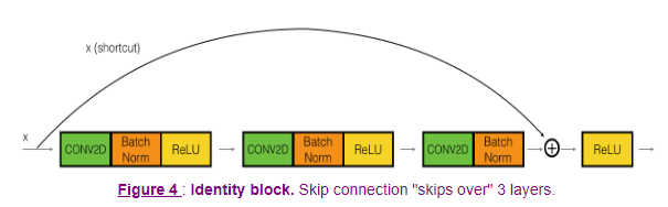
이 identity_block을 구현해 볼 것이다

앞서 강의에선 2개를 건너뛰었지만, 1 x 1을 이용한 3개의 레이어를 건너뛰는 블록을 구현할 것이다

def identity_block(X, f, filters, training=True, initializer=random_uniform):
    """
    Implementation of the identity block as defined in Figure 4
    
    Arguments:
    X -- input tensor of shape (m, n_H_prev, n_W_prev, n_C_prev)
    f -- integer, specifying the shape of the middle CONV's window for the main path
    filters -- python list of integers, defining the number of filters in the CONV layers of the main path
    training -- True: Behave in training mode
                False: Behave in inference mode
    initializer -- to set up the initial weights of a layer. Equals to random uniform initializer
    
    Returns:
    X -- output of the identity block, tensor of shape (m, n_H, n_W, n_C)
    """
    
    F1, F2, F3 = filters
    X_shortcut = X
    
    # First component of main path
    X = Conv2D(filters = F1, kernel_size = 1, strides = (1,1), padding = 'valid', kernel_initializer = initializer(seed=0))(X)
    X = BatchNormalization(axis = 3)(X, training = training) # Default axis
    X = Activation('relu')(X)
    
    ## Second component of main path
    X = Conv2D(filters = F2, kernel_size = f, strides = (1,1), padding = 'same', kernel_initializer = initializer(seed=0))(X)
    X = BatchNormalization(axis = 3)(X, training = training)
    X = Activation('relu')(X)
    ## Third component of main path
    X = Conv2D(filters = F3, kernel_size = 1, strides = (1,1), padding = 'valid', kernel_initializer = initializer(seed=0))(X)
    X = BatchNormalization(axis = 3)(X, training = training)
    
    ## Final step: Add shortcut value to main path, and pass it through a RELU activation
    X = Add()([X , X_shortcut])
    X = Activation('relu')(X) 
    
    return X

필터 크기나 conv가 valid, same인지는 요구하는 바에 맞춰 구현했고

형태만 보도록 하자 (shortcut은 최종 렐루 전에 적용된다!)

final step에서 tf의 Add()를 사용하지 않고, 그냥 더해서 과제에서 계속 에러가 발생했었다..

 

자 그런데, identity 하지 않고, shortcut에 conv를 줄 수도 있다

def convolutional_block(X, f, filters, s = 2, training=True, initializer=glorot_uniform):
    """
    Implementation of the convolutional block as defined in Figure 4
    
    Arguments:
    X -- input tensor of shape (m, n_H_prev, n_W_prev, n_C_prev)
    f -- integer, specifying the shape of the middle CONV's window for the main path
    filters -- python list of integers, defining the number of filters in the CONV layers of the main path
    s -- Integer, specifying the stride to be used
    training -- True: Behave in training mode
                False: Behave in inference mode
    initializer -- to set up the initial weights of a layer. Equals to Glorot uniform initializer, 
                   also called Xavier uniform initializer.
    
    Returns:
    X -- output of the convolutional block, tensor of shape (m, n_H, n_W, n_C)
    """
    
    F1, F2, F3 = filters
    X_shortcut = X
    ##### MAIN PATH #####
    
    # First component of main path glorot_uniform(seed=0)
    X = Conv2D(filters = F1, kernel_size = 1, strides = (s, s), padding='valid', kernel_initializer = initializer(seed=0))(X)
    X = BatchNormalization(axis = 3)(X, training=training)
    X = Activation('relu')(X)
    ## Second component of main path
    X = Conv2D(filters = F2, kernel_size = f, strides = (1, 1), padding='same', kernel_initializer = initializer(seed=0))(X)
    X = BatchNormalization(axis = 3)(X, training=training)
    X = Activation('relu')(X)
    ## Third component of main path
    X = Conv2D(filters = F3, kernel_size = 1, strides = (1, 1), padding='valid', kernel_initializer = initializer(seed=0))(X)
    X = BatchNormalization(axis = 3)(X, training=training)
    
    ##### SHORTCUT PATH #####
    X_shortcut = Conv2D(filters = F3, kernel_size = 1, strides = (s, s), padding='valid', kernel_initializer = initializer(seed=0))(X_shortcut)
    X_shortcut = BatchNormalization(axis = 3)(X_shortcut, training=training)
    
    # Final step: Add shortcut value to main path (Use this order [X, X_shortcut]), and pass it through a RELU activation
    X = Add()([X, X_shortcut])
    X = Activation('relu')(X)
    
    return X

shortcut을 더하기 전에 conv와 BatchNormalization이 적용된다

 

위에서 구현한 블록들로 50개의 레이어를 가진 ResNet모델을 만들어 보자

이렇게 생긴 애를 구현하자

def ResNet50(input_shape = (64, 64, 3), classes = 6):
    """
    Stage-wise implementation of the architecture of the popular ResNet50:
    CONV2D -> BATCHNORM -> RELU -> MAXPOOL -> CONVBLOCK -> IDBLOCK*2 -> CONVBLOCK -> IDBLOCK*3
    -> CONVBLOCK -> IDBLOCK*5 -> CONVBLOCK -> IDBLOCK*2 -> AVGPOOL -> FLATTEN -> DENSE 
    Arguments:
    input_shape -- shape of the images of the dataset
    classes -- integer, number of classes
    Returns:
    model -- a Model() instance in Keras
    """
    
    # Define the input as a tensor with shape input_shape
    X_input = Input(input_shape)
    
    # Zero-Padding
    X = ZeroPadding2D((3, 3))(X_input)
    
    # Stage 1
    X = Conv2D(64, (7, 7), strides = (2, 2), kernel_initializer = glorot_uniform(seed=0))(X)
    X = BatchNormalization(axis = 3)(X)
    X = Activation('relu')(X)
    X = MaxPooling2D((3, 3), strides=(2, 2))(X)
    # Stage 2
    X = convolutional_block(X, f = 3, filters = [64, 64, 256], s = 1)
    X = identity_block(X, 3, [64, 64, 256])
    X = identity_block(X, 3, [64, 64, 256])
    ## Stage 3
    X = convolutional_block(X, f = 3, filters = [128, 128, 512], s = 2)
    X = identity_block(X, 3, [128, 128, 512])
    X = identity_block(X, 3, [128, 128, 512])
    X = identity_block(X, 3, [128, 128, 512])
    
    ## Stage 4
    X = convolutional_block(X, f = 3, filters = [256, 256, 1024], s = 2)
    X = identity_block(X, 3, [256, 256, 1024])
    X = identity_block(X, 3, [256, 256, 1024])
    X = identity_block(X, 3, [256, 256, 1024])
    X = identity_block(X, 3, [256, 256, 1024])
    X = identity_block(X, 3, [256, 256, 1024])
    ## Stage 5
    X = convolutional_block(X, f = 3, filters = [512, 512, 2048], s = 2)
    X = identity_block(X, 3, [512, 512, 2048])
    X = identity_block(X, 3, [512, 512, 2048])
    ## AVGPOOL
    X = AveragePooling2D(pool_size=(2,2))(X)
    
    # output layer
    X = Flatten()(X)
    X = Dense(classes, activation='softmax', kernel_initializer = glorot_uniform(seed=0))(X)
    
    
    # Create model
    model = Model(inputs = X_input, outputs = X)
    return model

뭔가 무지성 복붙이라 맘에 안 드는데, 이렇게 하라니까...

위와 동일하게 형태만 보도록 하자

 

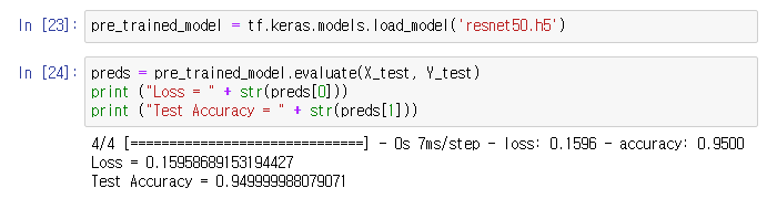
모델을 만들었으니, 뭔가 셋에 돌려보자

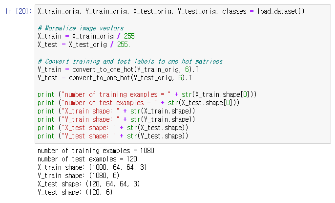
그런데 파일이 없으니 과제 캡처로 대체한다

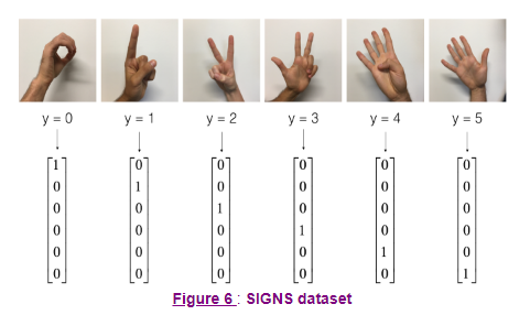
손동작 이미지

손동작 이미지 셋을 train/test 셋으로 쪼개고 학습시킨다

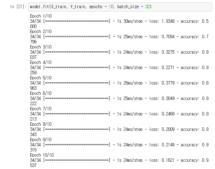
야호

오픈소스 어디선가 모델을 잘 주워와 사용한 결과도 좋다고 한다

---

다음으로 MobileNet을 이용한 Transfer Learning을 배워보자

data augumentaion이나 전처리는 넘어가자

우리의 모델에 다음과 같은 bottleneck block을 넣을 것이다

IMG_SHAPE = IMG_SIZE + (3,)
base_model = tf.keras.applications.MobileNetV2(input_shape=IMG_SHAPE,
                                               include_top=True,
                                               weights='imagenet')

위와 같이 기존의 모델을 base_model로 설정하자

자 그런데 위의 모델을 그대로 테스트 set에 적용해 보면 아래와 같은 이상한 결과가 나온다

base_model.trainable = False
image_var = tf.Variable(preprocess_input(image_batch))
pred = base_model(image_var)

tf.keras.applications.mobilenet_v2.decode_predictions(pred.numpy(), top=2)

일부 캡쳐

이상한 동물들만 잔뜩 나오고, 심지어 알파카는 없다

당연하게도 기존의 softmax는 알파카/알파카 아님으로 분류하는 것이 아닌, 동물 분류기 였기 때문이다

우리는 이를 잘 작동하게 만들기 위해 적어도 softmax 층은 변경을 해줘야 한다

자 그럼 먼저 최종 softmax만 학습하는 알파카_모델을 만들어보자

def alpaca_model(image_shape=IMG_SIZE, data_augmentation=data_augmenter()):
    ''' Define a tf.keras model for binary classification out of the MobileNetV2 model
    Arguments:
        image_shape -- Image width and height
        data_augmentation -- data augmentation function
    Returns:
    Returns:
        tf.keras.model
    '''
    
    
    input_shape = image_shape + (3,)
        
    base_model = tf.keras.applications.MobileNetV2(input_shape=input_shape,
                                                   include_top=False, # <== Important!!!!
                                                   weights='imagenet') # From imageNet
    
    # freeze the base model by making it non trainable
    base_model.trainable = False 
    # create the input layer (Same as the imageNetv2 input size)
    inputs = tf.keras.Input(shape=input_shape) 
    
    # apply data augmentation to the inputs
    x = data_augmentation(inputs)
    
    # data preprocessing using the same weights the model was trained on
    x = preprocess_input(x)
    
    # set training to False to avoid keeping track of statistics in the batch norm layer
    x = base_model(x, training=False) 
    
    # add the new Binary classification layers
    # use global avg pooling to summarize the info in each channel
    x = tf.keras.layers.GlobalAveragePooling2D()(x)
    # include dropout with probability of 0.2 to avoid overfitting
    x = tf.keras.layers.Dropout(rate=.2)(x)
        
    # use a prediction layer with one neuron (as a binary classifier only needs one)
    outputs = tf.keras.layers.Dense(1)(x)
    
    model = tf.keras.Model(inputs, outputs)
    
    return model

"include_top=False"을 속성으로 주어 최종 출력 층을 제거한 모델을 가져오고,

"base_model.trainable = False" 줄을 이용하여, 모델의 파라미터를 변경되지 않도록 만들었다

또한 이진 분류 출력층을 제작하여 알파카/비알파카 분류기를 제작하였다

학습하고, set을 돌려보면 아래와 같은 결과가 나온다

그럭저럭 괜찮아 보이지만, FIne-tuning을 적용하여 정확도를 더 높일 수 있다

base_model = model2.layers[4]
base_model.trainable = True
# Fine-tune from this layer onwards
fine_tune_at = 120
# Freeze all the layers before the `fine_tune_at` layer
for layer in base_model.layers[:fine_tune_at]:
    layer.trainable = False
    
# Define a BinaryCrossentropy loss function. Use from_logits=True
loss_function=tf.keras.losses.BinaryCrossentropy(from_logits=True)
# Define an Adam optimizer with a learning rate of 0.1 * base_learning_rate
optimizer = tf.keras.optimizers.Adam(learning_rate=0.1 * base_learning_rate)
# Use accuracy as evaluation metric
metrics=['accuracy']
model2.compile(loss=loss_function,
              optimizer = optimizer,
              metrics=metrics)

un-freeze한 레이어를 늘려 학습을 시작했다

낮은 레이어의 선 찾기, 면 찾기와 달리 복잡한 새로운 특성을 학습시켜준 느낌이다

그러자 이전보다 모델의 성능이 향상된 점을 알 수 있다

물론 학습 시간이 더 오래 걸리기에, 적절히 해줘야 한다